Getting Started

SimAPI in an OnScale Solve Scripted Study

This guide describes the python interface for SimAPI and how it can be used through the Scripted Study interface of OnScale Solve.

The Scripted Study interface provides a python editor for SimAPI and a live link between the SimAPI code entered and Solve’s graphical simulation interface.

Here, we will generate a SimAPI script for the static deflection of an I-beam and then modify to apply a distributed load with an expression.

The Scripted Study interface can be opened from the < > icon on any page of the Solve Modeler.

The generated SimAPI code for the current simulation can be viewed and edited within the Scripted Study window. The command reference for SimAPI python describes all of the currently supported SimAPI features and parameters. New simulation features can be added to the SimAPI code, validated and saved. If the added features are supported by the graphical interface they will display when the Scripted Study window is closed. Other valid features that are supported by SimAPI, but not yet by Solve will be included in the simulation, but not displayed in the graphical interface.

I-beam example with distributed load

Import the geometry into Solve

The I-beam CAD model can be downloaded here. Log into OnScale Solve and import the I-beam model.

In the Modeler view set the material to Structural Steel
In the Physics view apply a restraint condition on minimum-Y face (Face 13) with X, Y and Z restrained.
In the Physics view apply a traction downward on the top surface (Face 11) with magnitude of 1e6 Pa.

traction downward on top surface

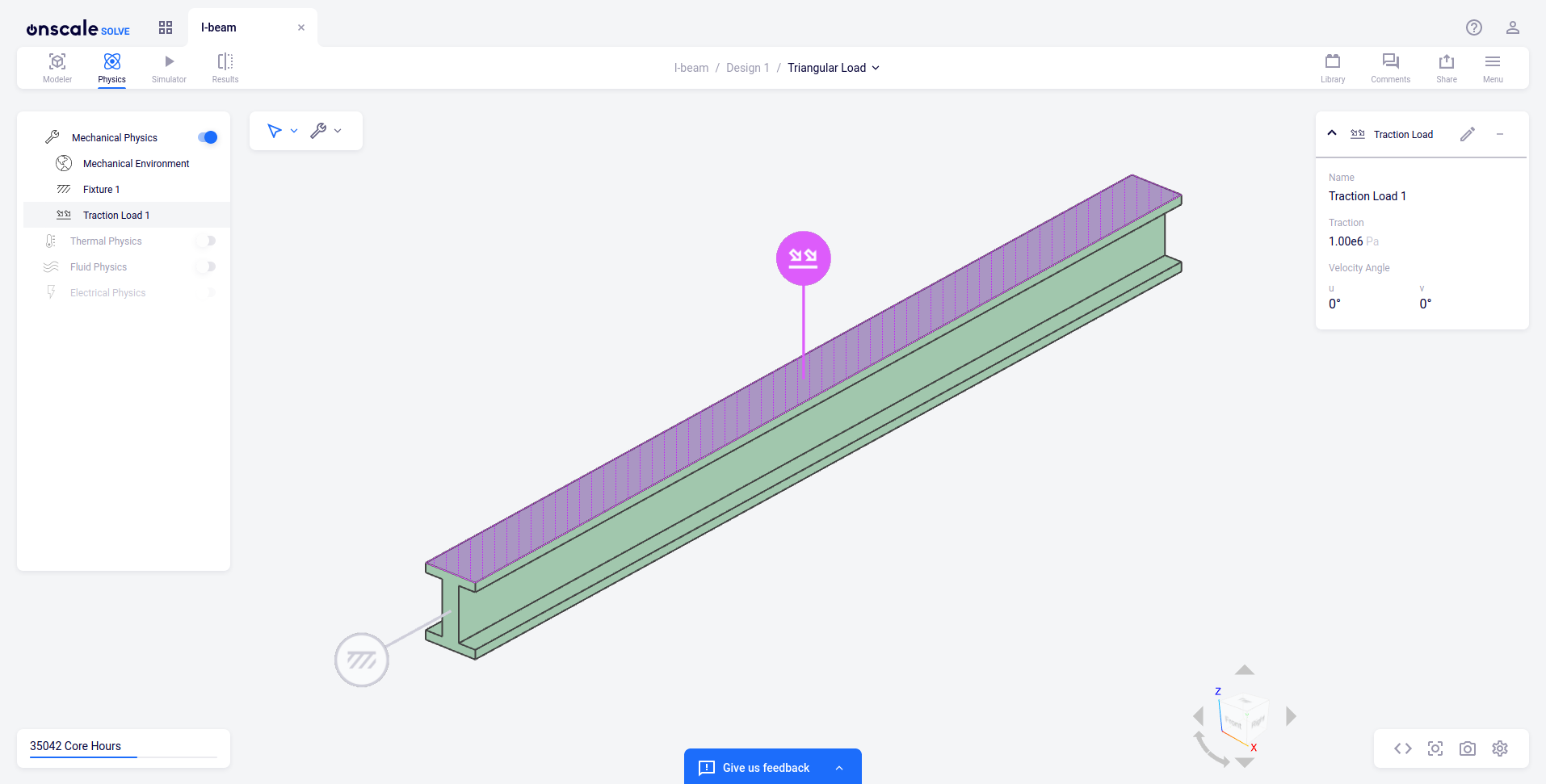
Open the Scripted Study interface

Open the Scripted Study window by clicking the < > icon. The interface opens in read-only mode. The SimAPI code should look like this:

"""
    Auto-generated simulation code.
"""
import onscale as on

with on.Simulation('None', '') as sim:

    # General simulation settings
    on.settings.DisabledPhysics(["thermal", "fluid", "electrical"])

    # Define geometry
    geometry = on.CadFile('i-beam.step', unit="m")

    # Define material database and materials
    materials = on.CloudMaterials('onscale')
    structural_steel = materials['Structural steel']
    structural_steel >> geometry.parts[0]

    # Define and apply loads
    restraint = on.loads.Restraint(x=True, y=True, z=True, alias='Fixture 1')
    restraint >> geometry.parts[0].faces[13]
    traction = on.loads.Traction(1000000, [0, 0, -1], alias='Traction Load 1')
    traction >> geometry.parts[0].faces[11]

    # Define output variables
    probe = on.probes.ResultantForce(geometry.parts[0].faces[13])
    on.fields.Displacement()
    on.fields.Stress()
    on.fields.Strain()
    on.fields.VonMises()
    on.fields.PrincipalStress()
    on.fields.PrincipalStrain()

Let’s look at each line of code.

The onscale module containing the Simulation API is loaded at the top of the file.

import onscale as on

A Simulation object is created to contain the simulation description. Here the optional name is defaulted to 'None'. Other python modules can also be imported, for example numpy.

with on.Simulation('None','') as sim:

Individual physics can be deactivated through the settings node. This allows multiphysics features to be included in the file without considering them in a particular simulation.

    # General simulation settings
    on.settings.DisabledPhysics(["thermal", "fluid", "electrical"])

A geometry object is created from an imported CAD file. Features of this geometry will be referenced by other objects in the simulation.

    # Define geometry
    geometry = on.CadFile('i-beam.step', unit="m")

A material definition database is first loaded into a materials object, in this caes from the OnScale cloud repository. The material ‘Structural steel’ is selected from the database as the structural_steel object.

    # Define material database and materials
    materials = on.CloudMaterials('onscale')
    structural_steel = materials['Structural steel']

structural_steel is applied to a part in the geometry. The binary >> operator is used to apply A to B (A >> B). In this simulation, there is a single part easily identified as geometry.parts[0], however it is also possible to reference parts by metadata tags if they have been assigned in the CAD file.

   structural_steel >> geometry.parts[0]

Boundary conditions and loads are defined with the loads node. Here a restraint with all degrees-of-freedom fixed is defined and applied to part 0, face 13.

    # Define and apply loads
    restraint = on.loads.Restraint(x=True, y=True, z=True, alias='Fixture 1')
    restraint >> geometry.parts[0].faces[13]

Similarly, we can define a traction with a magnitude of 1,000,000 Pa is the negative z-direction and apply it to part 0, face 11.

    traction = on.loads.Traction(1000000, [0, 0, -1], alias='Traction Load 1')
    traction >> geometry.parts[0].faces[11]

Simulation outputs can be requested as either probes or fields data. probes output as either a scalar or a time-dependent trace and can include either single point values or aggregates of field data. fields are output as multidimensional contours plotted on the geometry. First, a probe of the force resultant on the restrained face is requested.

    probe = on.probes.ResultantForce(geometry.parts[0].faces[13])

Finally, several field contours are requested.

    on.fields.Displacement()
    on.fields.Stress()
    on.fields.Strain()
    on.fields.VonMises()
    on.fields.PrincipalStress()
    on.fields.PrincipalStrain()

Modify the SimAPI code to apply a triangular-shaped distributed load

To enable editing, click on the pencil icon in the top right corner.
Add an expression to the traction definition representing the triangular-shaped load. The load \(`p`\) (with units of N/m\(`^2`\)) has a maximum value \(`p_0`\) at the fixed end of the beam \(`y = -0.5`\) m and decreases to zero at the free end \(`y = 0.5`\) m.

\[p = p_0 * (0.5-y)\]

traction = on.loads.Traction(f'1.0e6*(0.5-y)', [0.0, 0, -1], alias='Traction Load 1')

Add a probe point at the free end of the beam to record the deflection.

point = on.Point(0, 0.5, 0)
probe_2 = on.probes.Displacement(point)

The SimAPI python should look like this after these edits.

"""
    Auto-generated simulation code.
"""
import onscale as on

with on.Simulation('None', '') as sim:

    # General simulation settings
    on.settings.DisabledPhysics(["thermal", "fluid", "electrical"])

    # Define geometry
    geometry = on.CadFile('i-beam.step', unit="m")

    # Define material database and materials
    materials = on.CloudMaterials('onscale')
    structural_steel = materials['Structural steel']
    structural_steel >> geometry.parts[0]

    # Define and apply loads
    restraint = on.loads.Restraint(x=True, y=True, z=True, alias='Fixture 1')
    restraint >> geometry.parts[0].faces[13]
    traction = on.loads.Traction(f'1.0e6*(0.5-y)', [0, 0, -1], alias='Traction Load 1')
    traction >> geometry.parts[0].faces[11]

    # Define output variables
    probe = on.probes.ResultantForce(geometry.parts[0].faces[13])
    on.fields.Displacement()
    on.fields.Stress()
    on.fields.Strain()
    on.fields.VonMises()
    on.fields.PrincipalStress()
    on.fields.PrincipalStrain()

    point = on.Point(0, 0.5, 0)
    probe_2 = on.probes.Displacement(point)

Click Build in the bottom right corner to validate. If the code validates, the Build button will change to say Save. If there are errors they will be reported in the Console window.
Click Save to save the added features and return to the Solve graphical interface.

Note that following Build and Save, SimAPI may reformat some of the newly added code for style consistency.

Simulate

Proceed to the Simulator view. Mesh & Estimate, then Run.

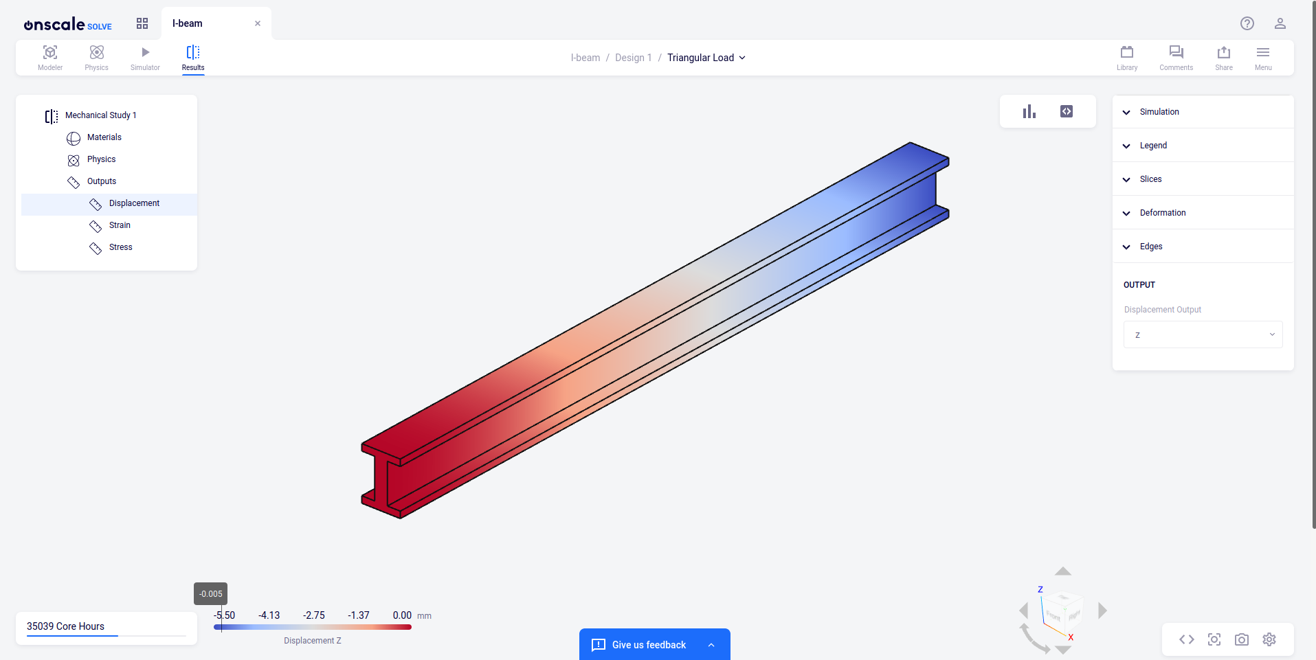
Post-process results

Contour Plots A field plot of the displacement in the z-direction shows a maximum deflection of -5.5 mm at the free end of the beam. This result can be validated by comparing it against an analytical solution for this simple configuration. Euler-Bernoulli Beam Theory (which does not account for the effects of transverse shear strain) predicts a deflection of -5.43 mm validating the simulation results that do account for shear.

scripted study read-only mode

Scripted post-processing in Jupyter Notebook The built-in Jupyter Notebook provides a versatile way to analyze results on the cloud without downloading. We can check and operate on the probe results directly in the Jupyter Notebook interface.

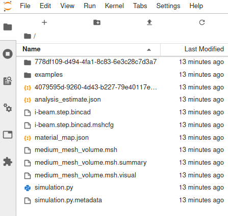
Open a Notebook by clicking the icon in the top right corner.
Simulation files are shown in the tree on the left side:

Simulation results are stored in the /simulationID/output subfolder (where simulationID is an alpha-numeric string):

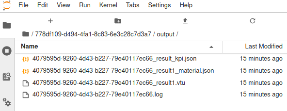
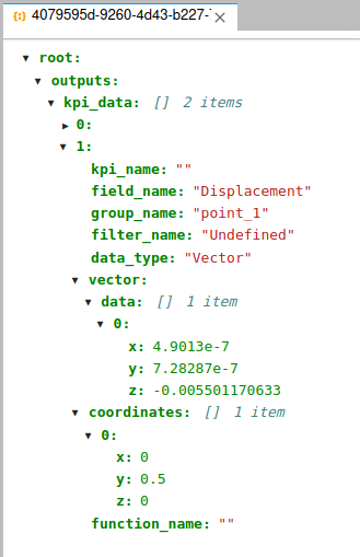
Probe results are stored in the simulationID_result_kpi.json file. Here we see that the end deflection computed is -0.005501 m in the z-direction.

I-beam example variations

Define a local coordinate system for the load

In the I-beam example above it was trivial to shift the expression for the triangular load to line up with global coordinate system origin that is positioned 0.5 m along the length of the beam in the y-direction. However, for many geometries it may be necessary to define an expression using a local coordinate system. Here we can create a local coordinate system with its origin at the fixed end of the beam:

    # Coordinate systems
    cs_1 = on.CoordinateSystem(vector_1=[1,0,0], vector_2=[0,1,0], center=[0,-0.5,0], system_type='Cartesian')

… and modify the traction definition to use the local y-coordinate:

traction = on.loads.Traction(f'1.0e6*(1-{cs_1.y})', [0, 0, -1], alias='Traction Load 1')